Vue normale

Reçu avant avant-hier

A Class on Predicting FM Radio Signals

21 avril 2026 à 14:00

Nick’s Signal Spot is a new feature in which Nick Langan explores RF signals, propagation, new equipment and related endeavors. 

At Villanova University, I teach an undergraduate Computer Science course, Platform-Based Computing (CSC 2053).

It is a fun class and one I feel fortunate to be able to instruct. The first half covers web and mobile application development, which for at least many of the students is their first time building applications. The second half then takes my students through many of the cool things they can do with the Python programming language.

Python is well-known in the data science community for its adaptability to large datasets, breaking them down statistically and gathering potential trends, and then, in some cases, to make predictions.

My 16 students by now are probably good and tired of looking at radio station data — but I jumped at the chance to use real-world data that I’ve gathered for my RadioLand app project.

After a few weeks of using Python libraries to make some general observations on radio stations in a given state that they chose, I wanted to see if we could come up with a way to predict the signal strengths, or field strengths, of FM stations, numerically.

Machine learning is a way to train software, known as a model, to make predictions using data.

The data generated by the time-tested Longley-Rice propagation model, still relied upon by the FCC and many others and used within my RadioLand app, would work as the perfect training dataset for the class.

The study

A course on machine learning itself could easily span a whole semester. For me, I only had one two-and-a-half-hour class to explore it with the group and some of that time was devoted to their ongoing semester-long projects.

So, the most practical approach was to explore the use of a common first-time machine learning tactic: predicting through linear regression.

In its most basic form, linear regression is a technique that finds a relationship between statistical variables. In the context of our lab, we wanted to find which statistics have the strongest relationship to predict an FM station’s field strength.

I extracted out of my RadioLand server pre-calculated Longley-Rice data for 25 random locations across the United States, with the signals measured in dBuV/m.

You can see a map of those locations below.

In the CSC 2053 lab, we used 25 random U.S. locations with previously generated Longley-Rice signal predictions.
In the CSC 2053 lab, we used 25 random U.S. locations with previously generated Longley-Rice signal predictions. I used Python’s Folium library to generate the map you see above. Click to enlarge.

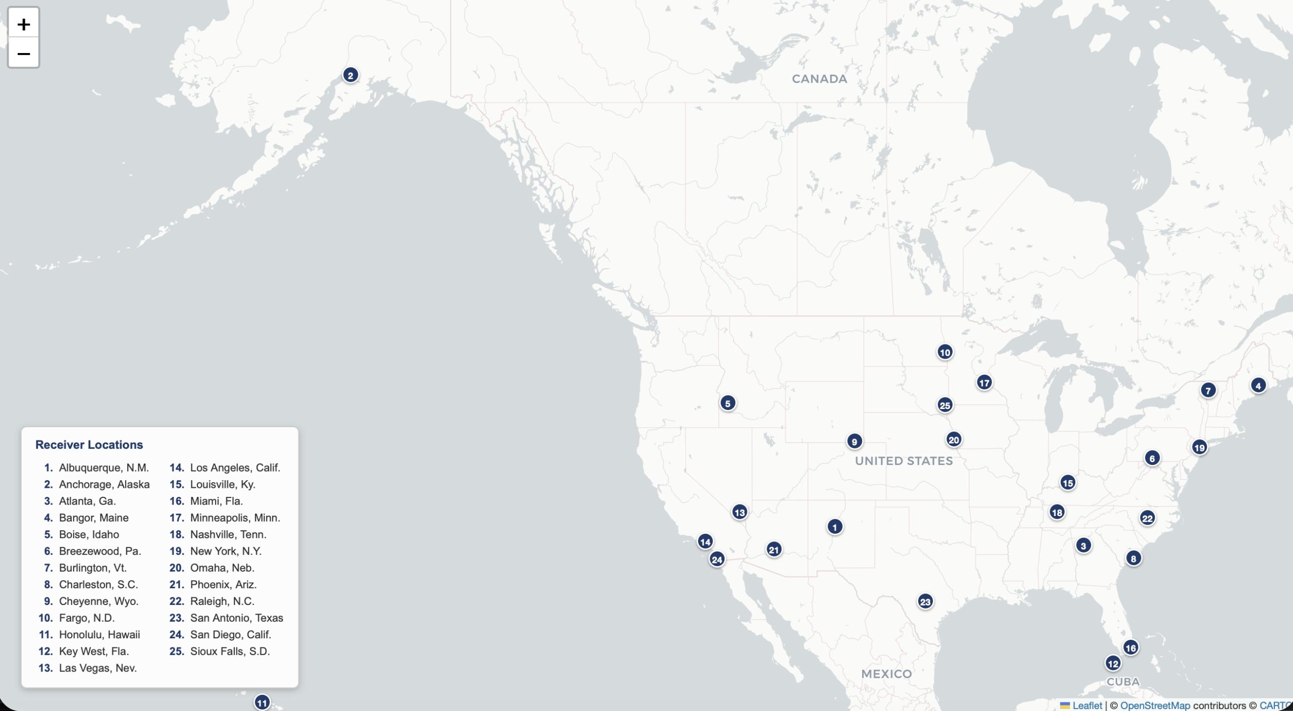
For each location, we had all FM stations available that Longley-Rice predicted to have field strengths of at least 40 dBuV/m. Then, we also had each station’s callsign, frequency, city, state, transmitting effective radiated power, antenna height above average terrain and the distance from our “receiver” location.

80/20 rule

First, I had the students run through typical machine learning techniques, which include splitting our 25-city data into “test” and “training” datasets.

The training data — or 80% of it — is used to train our linear regression model.

The test data — or the remaining 20% — is used to test the model to see how accurately it performs. The logic behind it is akin to knowing the answers to a test ahead of time.

That’s something my students can appreciate!

A model can perform well on the data it knows, but what happens when we throw it curveballs?

This all might sound complicated, but Python’s scikit-learn library has a linear regression model built right in. With programming syntax under our belt, it’s more a matter of feeding it the data and analyzing its performance.

Distance-first approach

With just a rudimentary understanding of signal propagation, you can probably discern that the most logical place to start for testing a feature’s relationship to predicting the strength of a radio signal is the distance from the transmitter.

The farther you are away from the source, the weaker it ought to be.

So that’s where we started. Could distance alone be a reliable predictor of a station’s field strength?

With our regression model, we use a metric called the R-squared score to understand its performance. Depending on the situation, it’s a quick and easy way to score the effectiveness of the relationship between our features and what we are trying to predict.

An R-squared score of 1 is a perfect score. A score of 0.5 would mean our feature explains half of the variance that is possible with our target. In some cases that might be OK.

But with field strength, we wanted to aim for something higher.

In our first go-around just using the distance, it resulted in an R-squared score of 0.48.

With linear regression, we want our model to plot as close to the line pictured. In this case, because the data is so scattered, it shows that distance from a transmitter alone does not predict a station's field strength.
With linear regression, we want our model to plot as close to the line pictured. In this case, because the data is so scattered, it shows that distance from a transmitter alone does not predict a station’s field strength.

Scikit-learn also provides us with the root mean squared error, which gives us the average magnitude of error between the predicted and actual values in the exact same units we are trying to measure — dBuV/m. For our first regression model, it was about 16 dBuV/m.

That could be the difference between predicting a comfortably strong signal from a signal off the Empire State Building in New York City — at a level of 70 dBuV/m — and a fringe-type signal at around 55 dBuV/m.

To provide my students context, I gave them this very rough guide for measuring the quality of an FM signal strength in dBuV/m.
To provide my students context, I gave them this rough guide for measuring the quality of an FM signal strength in dBuV/m.

While there is indeed a relationship between distance and field strength, it is not strong enough on its own.

With a model, we can combine the predictive features. What happened if we added a station’s transmitting power, antenna height and frequency to the mix?

Our R-squared score improved to 0.74.

Distance has the strongest correlation, but second is ERP. Antenna height above average terrain and the station’s frequency itself showed a very weak relationship.

Fitting a line

A comparison of our three linear regression model attempts, using r-squared score.

You do not have to be a mathematical maven to explore computer programming or machine learning. But in some cases, a little know-how helps.

Linear regression is based on how well your predictive data fits along a straight line.

But radio signals follow the inverse-square law, which states that intensity is inversely proportional to the square of the distance from a source.

To engineer a feature that accounts for this, we have to address the non-linear relationship. A common and highly effective tactic in machine learning to “fit” non-linear data around a straight line is to take the logarithmic value of a feature — in this case, distance.

We added the log of the distance as well as the log of ERP, as that feature also has a non-linear relationship with the field strength.

The result? An R-squared score of 0.89, or a mean error of 7.5 dBuV/m.

What’s missing?

Then I asked each of the students, in their lab workbook, to analyze two of the cities in the 25-city data set to see how our linear model worked in each location in isolation. First, they were given New York City and then they could choose one of the other 25 cities.

On a map, they could compare stations that the model under-predicted, over-predicted or placed within close proximity of Longley-Rice. A green dot here is good — that means the model came within 5 dBuV/m of Longley-Rice for the same station, such as the signals on the Empire State Building, for example.

The map plots the locations of each of the stations predicted by our linear regression model. A green dot means the model underpredicted the station versus Longley-Rice. A red dot means the model overpredicted it.
The map plots the locations of each of the stations predicted by our linear regression model. A green dot, here, was good, meaning the model predicted within 5 dBuV/m of Longley Rice. An orange dot means the model’s prediction was more than 5 dBuV/m compared with Longley-Rice. A red dot means the model underpredicted Longley-Rice.

Sophomore student Anthony Dell’Avvocato pointed out that many of the over-predicted signals from a theoretical receiver in New York were in the direction of northern New Jersey.

Many of my students call New Jersey home, including Dell’Avvocato, and its geography has been a theme of some of our exercises all semester long.

“The model is struggling with urban canyons, terrain blocking and signal reflections, which aren’t captured by distance, power or height alone,” he wrote.

I finally asked each student if they were a broadcast engineer, would they find this model valuable?

Freshman Alan Uribe identified that although the Longley-Rice data it was trained on accounts for terrain, our linear model has no feature that does the same.

“It’s useful for early planning but not accurate enough for final decisions,” he said.

Sophomore Jack Behringer noted that for flatter areas, our regression model might prove useful. But in an area like California, he said, it would be thwarted by terrain.

“A real broadcast engineer knows the terrain and population of the area — this is overlooked by the model,” freshman Erin Campbell noted.

Takeaways

I don’t think anyone would comfortably rely on the model we came up with in one class to make real-world decisions. But the world of machine learning offers many more possibilities.

My research student, senior Minh Bigting, used a gradient boost model on similar data and has come up with promising results.

All in all, it was a fun way to show my group of students how FM signals travel and why there are a number of factors involved with hearing a station.

Comment on this or any article. Email radioworld@futurenet.com.

The post A Class on Predicting FM Radio Signals appeared first on Radio World.

Echo App Brings the Power of SDRs Into Your Pocket

7 avril 2026 à 17:00

Nick’s Signal Spot is a new feature in which Nick Langan explores RF signals, propagation, new equipment and related endeavors. 

In just the last year, Radio World has covered several different software-defined radio platforms.

Our James Careless recently profiled how KiwiSDR, WebSDR and OpenWebRX are bringing shortwave stations into your own home via remote receivers.

Meanwhile, for FM broadcast hobbyists like myself, there is the growing FMDX.org webserver project — a network I’m proud to participate in as a host.

If you’re new to the world of SDRs, however, the pace of development can be understandably dizzying. Where do you even begin?

We recently discovered a new mobile app that attempts to bridge this divide. Developed by Mark Garrison Jr., the Echo app brings four popular SDR platforms to your Apple iPhone or iPad. Garrison Jr.’s motivation for building the app is something I can appreciate and I’ve loved using it so far.

You can download Echo for free on iOS here, and I asked him some questions about the project in my latest Signal Spot.

Walkie-talkie childhood

Garrison with his wife, Maricarmen. He said he dedicated the Echo app to her. "Her support was absolutely crucial while I was building this over the last several months," he said.
Garrison Jr. with his wife, Maricarmen. He said he dedicated the Echo app to her. “Her support was absolutely crucial while I was building this over the last several months,” he said.

Garrison Jr., a 27-year-old pharmacy technician in Texas, has been a radio hobbyist since childhood.

Despite being firmly in the Gen-Z demographic, he owned a walkie-talkie long before he had a cell phone. “I used to love helping my father test long-range reception with his homemade antennas, seeing if I could hear him all the way from the town grocery store,” Garrison Jr. told us.

That experience planted the seed, but as he grew older, his biggest hurdle was the barrier to entry created by the cost of traditional equipment.

Eventually, he and his father discovered SDRs. Garrison Jr. was amazed that a small laptop, a $25 USB dongle and a magnetic antenna with an application like SDRTrunk could replicate the performance of a $1,000 digital scanner.

The Echo app uses a server in Austin to hear WWV's signal on 10000 kHz.
The Echo app uses a server in Austin to hear WWV’s signal on 10000 kHz.

It sparked a question: Could he harness the power of existing SDR networks and develop a mobile solution, something akin to many of the scanner apps that exist, but truly designed for a smartphone?

“I wanted something made for iOS that felt like ‘Apple quality’,” he said.

Garrison Jr. wrote Echo in Apple’s native Swift language to ensure a similar experience across iOS, iPadOS and macOS.

While development began last June as a personal project, he quickly realized there was a demand for a polished client that aggregated KiwiSDR, OpenWebRX, WebSDR and FMDX.org servers.

He was also careful to respect the community’s roots, speaking directly with KiwiSDR creator John Seamons and OpenWebRX developer Jakob Ketterl to ensure proper attribution.

The community’s response was, well, swift: A crowdfunding effort funded his Apple Developer license within ten minutes. After a two-month TestFlight beta with 200 users, Echo officially launched for iOS on March 31.

The iOS version is also available in the European Union. An Android version, he said, is also in development.

How it works

The beauty of Echo is that it doesn’t reinvent the wheel. There are so many SDR servers publicly available. A thoughtfully designed interface that can more easily bring them to you would go a long way. And that’s what I’ve found Echo is in my own use.

Echo can automatically match you with the nearest SDR server via location permissions or allow for manual selection.

If you tap the "Signal" button while connected to a server in the Echo app, it fetches space weather from NOAA to display a solar signal forecast.
If you tap the “Signal” button while connected to a server in the Echo app, it fetches space weather from NOAA to display a solar signal forecast.

Depending on your target — such as an FM broadcast station — Echo switches you to the appropriate platform.

When I asked Garrison Jr. what sets Echo apart, he highlighted these five areas:

  • The “smart scan” experience: Located in the main station tab, the feature allows users to cycle through categories like amateur radio frequencies, public safety and military bands. He said that of the user feedback he’s garnered so far, military bands have been the most popular.

  • On-demand flexibility: While the scanner mode is a highlight, Garrison Jr. also wanted Echo to mimic a true tuner. At any point, users can break out of a scan to focus on a specific frequency. This includes access to a “hot list” of popular selections.

  • Interactive map: “Users can filter by SDR type, physical distance or signal-to-noise ratio to ensure the best audio quality,” Garrison Jr. explained, which includes whether you want to hear something locally or from another country.

  • A smart manual tuner: Echo detects kHz vs. MHz and routes FM requests to the nearest FMDX.org server. “I’m particularly proud of how it handles server complexities,” Garrison said. “If a server doesn’t support a specific frequency, the app helps the user find a server that does.”

  • Global database: Echo uses a categorized database of over 11,000 frequencies. The list is constantly growing, Garrison Jr. said, covering everything from standard FM and amateur radio to spy-thwarting “numbers stations.”

Echo has already seen quite a few user-fueled modifications. Garrison Jr. recently added Apple VoiceOver support for blind and low-vision users. The project has an active Discord community that he encourages new users to join.

What a time to be alive

I’ve said this before and the Echo app is a reminder — there’s never been a better time to engage in the hobby of radio, whether it’s long-distance (DX) signal hunting or scanning.

There are smart, young people like Garrison Jr. that are catching the bug and using software development skills to aid our endeavors!

For me, I can’t wait to use Echo to aid my DX this upcoming E-Skip and tropospheric ducting listening this season.

[Read the Signal Spot from Nick Langan for More DX-Related Stories]

The post Echo App Brings the Power of SDRs Into Your Pocket appeared first on Radio World.

FM Autologging Made Easy

24 mars 2026 à 16:59

Nick’s Signal Spot is a new feature in which Nick Langan explores RF signals, propagation, new equipment and related endeavors. 

When I write about anything related to long-distance radio signal monitoring (DXing), it often comes attached with conflicting feelings.

Specifically, with my focus on the FM band, the dial has never been more crowded almost everywhere. You can still find some spots with a quiet RF noise floor, but you might have to drive a long time to get there.

But technology, in many ways, has never been better. Through software-defined radios, setup is simple, and with a decent receive antenna, you can capitalize when tropospheric ducting, e-skip or even meteor scatter opportunities cooperate.

In the past, timing really was everything. If an opening happened overnight, but you weren’t awake to hear it — unless you were running a cassette recording — as the old axiom goes, did it really even happen?

Now, since 2021, quite a few North American FM DXers are utilizing station RDS decodes to create a free, powerful autologger network, ensuring those overnight openings are no longer lost to the ether.

As of this writing, there are 86 active FM tuners online, from the Pacific Northwest in Seattle down to Bartow and Chipley, Fla., with representation in Alberta and Quebec, as well.

RabbitEars and TV bandscanning

The RabbitEars.Info all tuners FM map on a March morning.
This map from RabbitEars.Info shows all active FM tuners autologging in North America on a March morning.

You may already know the value of RabbitEars.Info. Founded in 2008 and operated by Mark Colombo, it is the definitive resource for U.S. TV station listings and searches, featuring a highly useful signal search map.

In 2013, Colombo added a live bandscan feature requiring an HDHomeRun receiver and an always-on computer to report real-time digital TV reception to a live map. The architect behind this service, however, is Russ Dwarshuis (KB8U).

Dwarshuis had originally written software back in 2009 to automatically log TV reception from a SiliconDust tuner to his own website to detect tropospheric ducting. Four years later, Colombo connected with Dwarshuis and offered to host the code on RabbitEars.Info, officially launching the live bandscan feature.

In 2021, Dwarshuis expanded the project, introducing a comparable feature for the FM band.

How the autologger works

Our friend Loyd Van Horn of DX Central put together a very helpful tutorial on how to use a TEF6686 receiver with the RabbitEars.Info FM reception map:

If you want to jump in, you can either use a software-defined radio that supports the SDR Console software, which means you’ll need both an SDR and a computer.

Alternatively, thanks to the efforts of Les Rayburn, you can also use a TEF6686 that runs Sjef Verhoeven (PE5PVB)’s firmware, which we’ve written about. No computer is needed for this setup — the TEF, via its built in Wi-Fi, can report directly to RabbitEars.Info.

Dwarshuis explained to us the mechanics of the FM logging system, which are fairly straightforward and rely on RDS. His software commands the radio to tune to each broadcast frequency for a few seconds, scanning from the bottom of the band to the top.

As it scans, it collects any available RDS Program Identification codes. Once the radio reaches the top of the band, a payload containing the frequency, PI code and the time of reception is sent to RabbitEars.info, tagged with the user’s ID.

From there, the server takes over, thanks to code authored by Dwarshuis. It references a database to find a callsign that matches both the reported frequency and the PI code, subsequently plotting the results on a live map. If multiple stations share the same PI code and frequency, the system defaults to logging the geographically closest match.

The primary reference for matching these frequencies and PI codes is the Worldwide TV-FM DX Association database, which the system polls once a week for updates. If no match is found there, the server falls back on other publicly available data.

Because the system plots received stations on the map for up to 24 hours, users can easily review what rolled in while the radio was left unattended.

I’ve had so many success stories doing this. You can view my autologger map here, and click the “ever received” button to see all logs back to 2021.

I’m coming up on the two-year anniversary of a memorable trip with my father to Boston. I couldn’t sleep in our hotel room, and around 3:00 a.m. one late March night, I checked my autologger, stationed in New Jersey, and saw that it was receiving tropospheric ducting signals down to South Carolina.

I hadn’t been expecting such propagation at all.

Current caveats

There’s been quite a bit of debate in DX circles on whether what the autologger detects should go directly into one’s logbook. It is a sensitive subject!

I always just resort to common sense in these cases, which admittedly, doesn’t seem to come easy these days.

A log from Hawaii captured in Maryland on a night in January probably didn’t happen. But if you’re getting other stations from Denver and the autologger finds 103.5 KRFX(FM), I’d say that’s a log!

Dwarshuis is realistic about the FM autlogger’s current weaknesses:

  • Incomplete RDS adoption: Not all FM stations transmit RDS data. Consequently, a significant number of stations simply fly under the radar and are not detected by the software.
  • Inaccurate station data: Stations occasionally transmit the wrong PI codes. When this happens, it requires manual corrections to the WTFDA database to ensure future logs are accurate.
  • False decodes: Even though the RDS protocol includes built-in error correction, the system is still susceptible to occasional false decodes, particularly when signals are weak or experiencing heavy interference.

He’s also sought an enhanced interface and encourages anyone with programming experience and passion to review its code on GitHub.

Getting involved

For those looking to join the free network, the community has streamlined the onboarding process. Rayburn has graciously agreed to set up accounts and provide configuration information specifically for users running TEF6686 radios, and he can be contacted directly for assistance.

Rayburn did caution that version 2.20.8 of the PE5PVB TEF firmware has a different connection setup for Wi-Fi, and Rayburn is working on adjusting his instructions for this process.

For DXers who prefer to use SDR Console, step-by-step setup instructions are available at the RabbitEars join page.

[Read the Signal Spot from Nick Langan for More DX-Related Stories]

The post FM Autologging Made Easy appeared first on Radio World.

❌